 JULIA Radar Homepage JULIA Radar Homepage
A large quantity of ionospheric irregularity data have been collected as part of the CEDAR MISETA campaign in the fall of 1996. There is also a significant amount of data from the years following. These data include daytime observations of the electrojet and 150 km echoes and nighttime observations of equatorial spread F. Data can be accessed through this site in graphical format. Researchers interested in acquiring the data in numerical format may contact the atmospheric physics group at Cornell University.
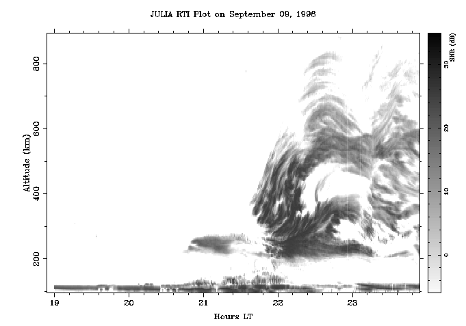
The benefits of unattended operations can be appreciated by looking at some early morning spread F data. RTI and drift data for a radar plume observed until shortly before sunrise are shown here. These very remarkable observations probably would not have been made had human intervention in the experiments been necessary. It now appears that such early morning events are commonplace.
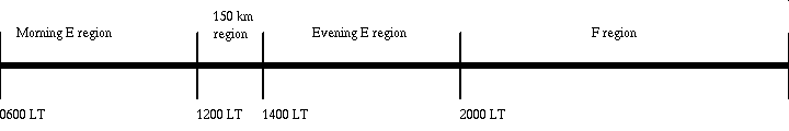
Here are several example plots from the different regions.
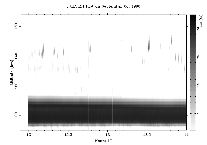
Example 150 km Region Plot
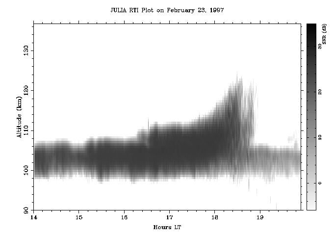
Example E Region Plot
Example F Region Plot
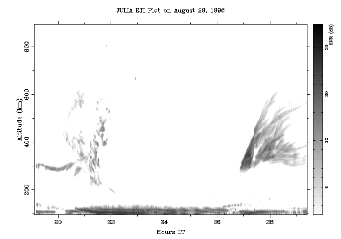
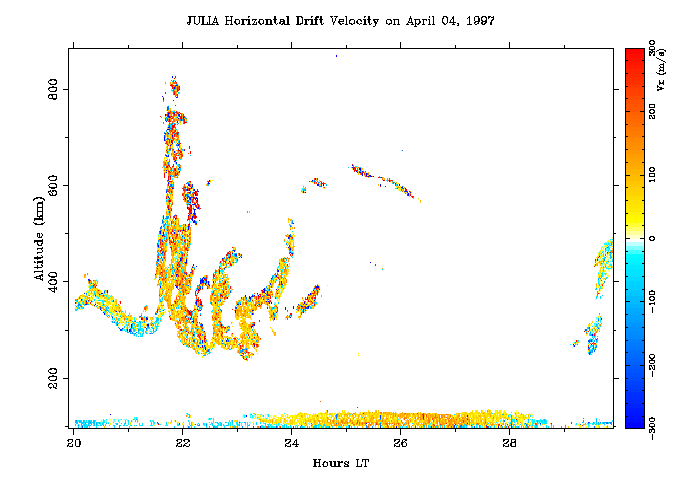
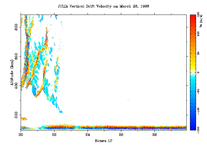
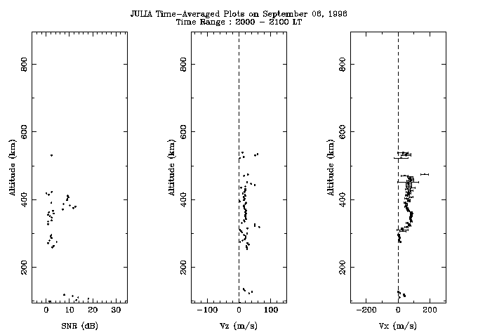
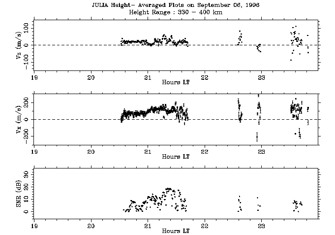
There are five possible plot types available which allow the user to examine the selected data in different ways. Signal to noise ratios are shown in conventional range-time-intensity (RTI) power map format. Horizontal and vertical drifts are shown with color coded speeds. Horizontal drifts are deduced by interferometry and positive values correspond to an eastward direction. On the vertical drift plots, upward vertical drifts are shown by positive values and represent Doppler phase speeds. If the OPTIONAL starting and ending times are entered, the plot only shows that time range. However, leaving the default "*"'s is usually the best choice! The last two plot types are the time-average plots and the height average plots. They show S/N ratios, horizontal drift speeds, and vertical drift speeds as three seperate plots. Each of the smaller plots are averaged over a specified region. The specified values must be times for the time-averaged plot and heights for the height-average plot. Example values are placed in the fields aleady. The three plots are presented in a single screen. Listed below are examples of the different plot types.
Example S/N Plot
Example Horizontal Velocity Plot
Example Vertical Velocity Plot
Example Time-Average Plot
Example Height-Average Plot
 Return to the
Space Science group homepage.
Return to the
Space Science group homepage.